Diffusion II
In this final project for CS180 Computer Vision and Computational Photography at UC Berkeley we were asked to develop a UNet based flow matching model on the MNIST Dataset of handwritten digits in 28x28 pixel format. This is a generative machine learning model that samples some input from random Gaussian noise and returns an iteratively "denoised" image ideally containing some visibly recognizable numeral.
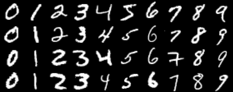
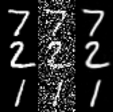
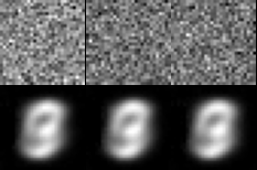
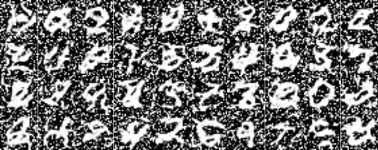
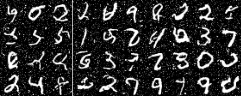
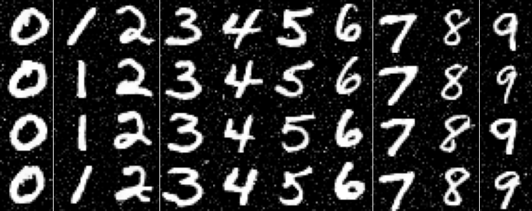
According to good practice, we start this journey by inspecting what our data looks like. The MNIST Dataset contains 70,000 handwritten grayscale digits labeled in classes 0 - 9. These digits are variable in form but are recognizable as the number they stand for. They're human handwriting! Something to notice is that some digits contain variations of structure - see the top two 2s and the third 7 as examples of this.
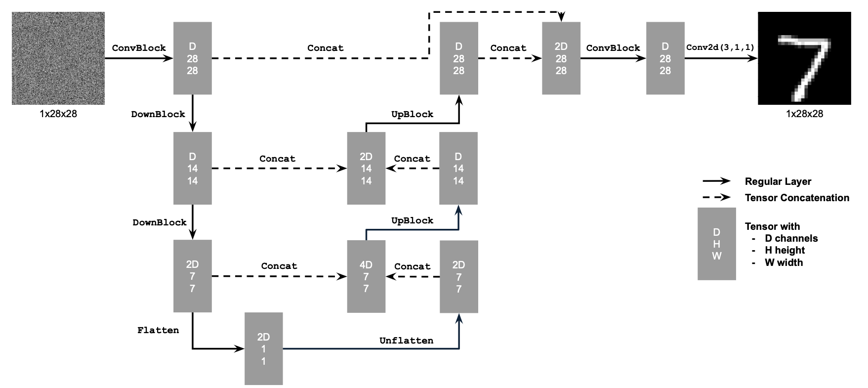
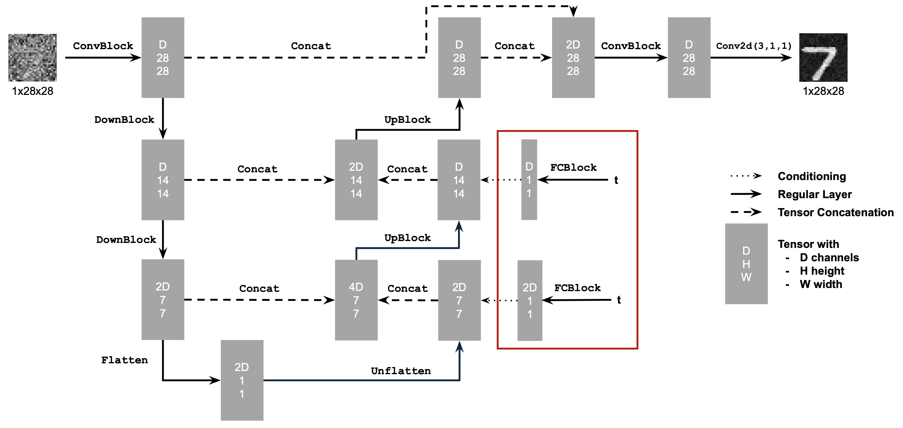
Given that dataset we wish to create some generative model that can interpret the structure of random Gaussian noise into a desired digit via an iterative process. This is a little much right off the bat. Instead, let's see if we can create a model that can interpret some noisy digit to some structure that aligns with the dataset. The architecture of this model can be found below and was built according to project specifications. This model is a conventional UNet with residual connections where the base premise can be thought of as a series of convolutional layers with downsampling to a small flattened layer which is upsampled back to the original size of our input/output. In each upsampling step we connect our new layer with the downsampled old of the same size with residual connections for ease of training.
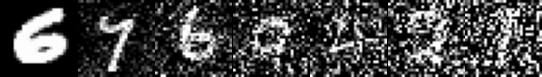
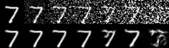
Let's go ahead and understand what exactly we're training upon. What is a "noisy" image? Below are 7 examples of noised images with different sigma (noise) values ranging from 0 (left) to 0.5 (middle) to 1 (right). This process is computed by finding some sample from the MNIST dataset, sampling some 28x28 Gaussian noise and adding some ratio of that noise (sigma) to our MNIST sample. You can see whatever digit is contained in the image below becomes less and less recognizable as it drifts to the right.
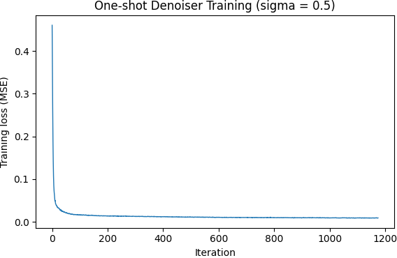
Let's go ahead and train our model on Mean Squared Error (MSE) loss between the output of the model upon noisy (sigma = 0.5) variations of the initial dataset and the MNIST data it is derived from. As you can see below, by epoch 5 (the fifth time the model has seen all training MNIST data) the model is able to very cleanly parse the noise away from the digit, despite different digits having a different inherent structure. The model is trained with Adam, lr 1e-4, batch size 256, and hidden dimension D = 128.
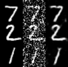
All fine and well, but let's investigate how this helps us generate from greater and greater amounts of noise. Remember - eventually we will be starting from pure noise. Below is an image of a seven digit with varying amounts of Gaussian noise added (0 to 1 left to right). The model performs well enough with less noise than it is trained upon but as noise increases the model hallucinates digit structure where nothing is liable to exist. This is indicative of Out-of-Distribution Testing. We were not trained to process this.
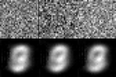
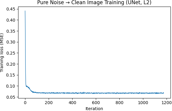
Can we train this model to handle pure noise and transform that noise into a legible digit? Unfortunately, that task is a little more complicated than this model can handle. As you can see below, the model learns to return the same blurry shape similar to an 8 with each variable noise input. This is a result of a couple factors: the model has to perform the denoising in one shot meaning it can't learn a nuanced flow and the loss function MSE means the model is incentivized to return some output that is between any and all possible MNIST digits. These factors combine to the blurry numeral 8 in the center of the output screen.
How can we elaborate our model to address the failures seen processing pure noise? We will see to the architecture and add two FCBlocks (small fully connected layers) as seen below. These additions will take in an arbitrary timestep t between 0 and 1 and use that to determine the incremental shift that the output image takes per step from pure noise / 0 to full resolution generated image / 1. The addition of time conditioning allows our model to learn more subtle flows that trace their way through the complex manifold of possible images to an output directly along the dataset manifold.
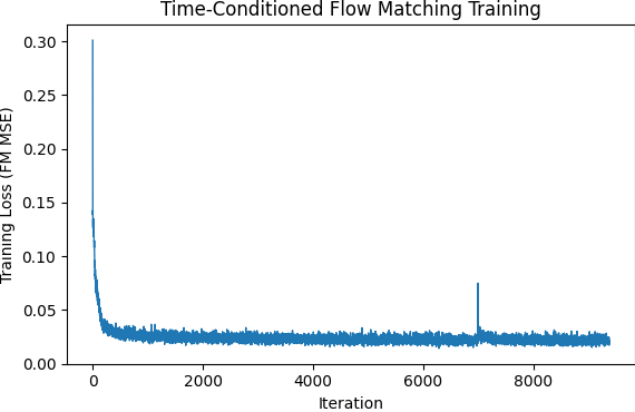
The next step is going to be training our newly conditioned model using the same dataset. How do we go about training what is essentially a time-defendant velocity field? For each iteration of training we sample three things: a sample from the MNIST dataset, a fully Gaussian noise sample, and some arbitrary timestep t. We calculate a ratio of noise to image dependent on t which we treat akin to the noised sample from Single Step Denoising UNet and optimize over the L2 loss between the model flow (eg velocity) that noisy sample would take to orient towards denoised version and the true flow calculated off our three initial samples.
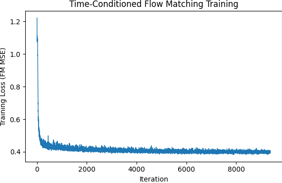
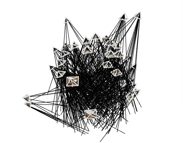
The first model trained in this manner was done so with Adam Update, an exponential decay lr starting at 1e-2 and decaying by 0.1 per epoch for a total of 10 epochs. The model was trained with batch size 64. Again we have shifted the output of the model from a single step denoise as final output image to the velocity this image takes per sample timestep iteration. We are approximating flow physics through the introduction of arbitrary timesteps.

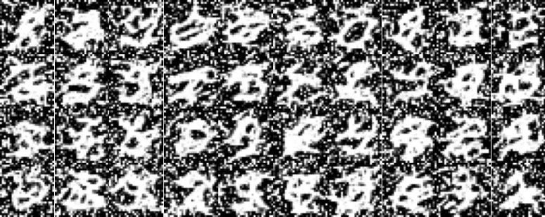
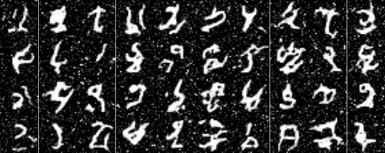
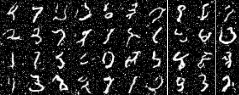
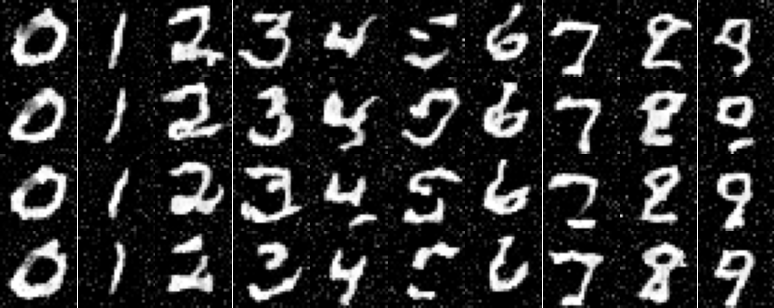
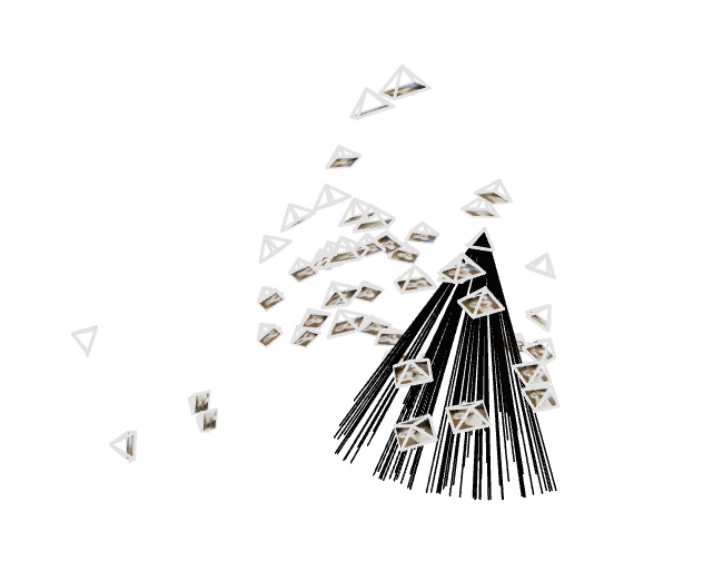
As you can see above the initial results I generated looked like hieroglyphs in a snowstorm. The model did not do so good of a job in reducing extraneous noise. The second attempt had me shift the sampled gaussian noise to have a variance of 0.3 compared to 1. This result still had a high degree of noise around the edges so later we shifted this to 0.2. We can see the presence of line structures that are sometimes recognizable as digits now! The model is trained in the same manner as above only a change in noise variance.
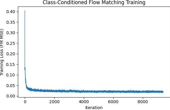
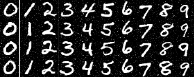
We will next implement a class conditioning system alongside the time conditioning system which will be present in training as well as sampling with classifier-free guidance set to 5.0 for clear distinctions. The class conditioning is set up extremely similarly to time conditioning with two additional fully connected blocks added in the same location and models trained to output numerals with accordance to the specified class - numeral type. We trained here with dropout 0.1 so as to reduce overreliance upon the class conditioning for structure.
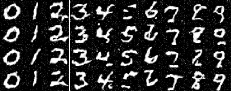
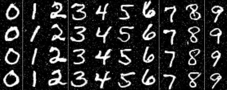
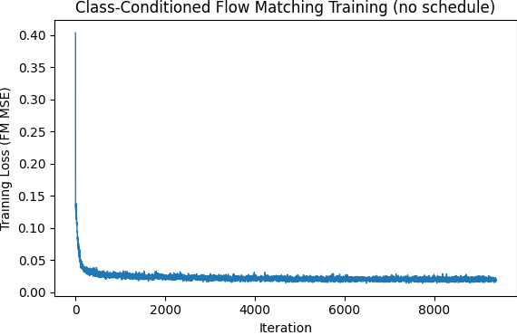
The final model we trained had us attempt to do without the exponential learning rate decay scheduler. Simplicity is best. To compensate for the loss of the scheduler we manually adjusted the learning rate by having two separate learning rates - initial and final - with initial at 1e-2 and final at 1e-3. At epoch 5 we wired a brief code switch changing the referenced learning rate. The outputs are rather similar to the ones above, but from my persepctive the exponential decay schedular had a better final epoch performance.
Diffusion
And another one. In this final project of my cs180 - Computer Vision and Computational Photography - class at UC Berkeley we were tasked with experimenting on the generated outputs of diffusion models in preparation for the creation of our own diffusion model built with Classifier Free Guidance (Transformer-style Flow Matching). The first section of this project involves an intuitive understanding of just how these models function - utilizing prompts and different noise samples in order to arrive at interesting engaging images. The second half has us building and training a flow-matching UNet upon the MNIST dataset.
Diffusion models are a modern way for computers to generate novel images - images that while they may look like they're taken by a human, are certainly not. These models are trained to transform sampled Gaussian noise into an image along it's learned "manifold" via an iterative denoising process. Before we experiment with the fundamentals of what that looks like, let's get a glimpse of what some of these images look like with an applicable prompt. This should be familiar to anyone who has generated an image with AI before. These are sampled with 20 steps of iterative denoising. I used random seed 42 for all my experiments and each image was generated using DeepFloyd IF-I-XL-v1.0 accessible off HuggingFace.


Neat. Let's check out the difference when we double the sampling steps (40) taken by the iterative denoiser. The following images are off the same prompt (and therefore pushed in the direction of the same manifold via context of CFG) but have a smoother alignment to the denoising process. We can see therefore there is a higher amount of detail contained within the below photos and they have more characteristics of the prompt.


Diffusion, like most learnable operations in machine learning, is broken up into a forward and backward process. Here specifically, the forward process takes a base image and iteratively adds noise to it so as to see the image go from legable to a collection of random gaussian pixels. We can define a timestep t that goes from 0 to 1 - base image to pure noise - and define a forward function below to generate images on a scale towards noise. Below the timesteps are from 0 to 1000 but they become unit normalized in preprocessing.


With each iterative forward step we need a way to return to the original image. Remember, our eventual goal is to go from randomly-sampled noise to images upon a manifold. A simple way to reduce this noise is to gaussian blur the image via convolution. As you can see visualized below, this is... not very good. As we get to higher amounts of noise, that noise overwhelms the signal and we end up just smearing everything together.


This is where the diffusion model comes into play. This model is trained to recognize patterns within noise, and aggregate pixels within the common lines of an image manifold - manifold being the surface of "good" images within the dimensionality of possible images generated with noise (a very very high dimension). If we run this model on the noisy forward passes generated above we regenerate a variation of the initial photo as seen below. These images are not the original image, some signal gets lost in the noise. More signal gets lost the greater the amount of noise. However, if we compare to the gaussian blur it's immesurably better.


But can we do a bit better? The last image is strange, there are masses of color that would have details in a true "realistic" photo. What if we iteratively denoise the original chaotic noise and allow for the introduction of new random noise in each iteration? This would allow the model to recognize major features in the first steps where there is overwhelming noise, but also allow the model to finetune its estimates when signal is more present. It allows the model to hallucinate detail and texture, two things we would expect to see in any realistic image. This detail doesn't necessarily match the original image, but if our goal is to generate novel images off of random noise this isn't a bug - it's a feature.
Below you can see the iterative denoising process at strided timesteps, as well as a final comparison between the three attempts we explored in cleaning the added gaussian noise off of a photo of Berkeley's Campanile.


In the last section we saw how to iteratively denoise an image. Extending this idea, let's start from fully random Gaussian noise. If we do so and iteratively denoise in the direction of the manifold of "natural" images we can iteratively generate an image from along this space. However, without any classification these images are generic and unlikely to be too much of a help to someone engaging with this model, this is akin to sampling from a diffusion model with a null prompt.


We now want to work with this process to create images that have a specific look and a higher quality, albeit for a drop in image diversity. To do this we use a process known as Classifier Free Guidance (CFG). Using a transformer architecture with learned directional embeddings for any inputted text prompt, we guide the iteratively generated image towards the manifold relating to that specific prompt. This supplants the process of introducing random noise the iterative process uses with noise sampled along the direction of the embeddings so that when the model aligns details it aligns those details in the direction of our prompt. Below are some examples of Classifier Free Guidance using the prompt "a high quality photo" with γ=7.


Classifier Free Guidance can be pretty interesting when used in conjunction with some of the earlier techniques we introduced - adding noise to an image and reversing that process to find a legible image. If we input a partially noised image to CFG, this process lets us derive images similar images along the manifold depending on where we begin the iterative process of denoising along steps i = 1 (first denoising step) to i = 20 (final denoising step). Below are some examples of the usage of this process, notice how images slowly drift away from the initial target - Campanile, Alarm, or Fire - as the iterate step we start at is reduced. Something else I noticed and found frustrating in this process was just how often the diffusion model wanted to hallucinate a photo of a woman instead of whatever we were attempting to generate. The prompt used in this denoising process was "a high quality photo" and γ=7 (how strong the pull towards prompt).


This process is especially interesting when used with images that themselves are not along this manifold, namely artistic renderings drawn with a Google Colab tool or sampled from the internet. We can see how the Diffusion model interprets a variety of shapes and colors and what the model considers a hallmark of an image along the correct manifold. Some of my favorite results I created were along the i5 initilization - it seems a great place to give inspiration to the model with shape and color without letting the model just go off and hallucinate some random woman.


A third use of this process is the creation of stylized images off of an initial image which is concattenated with noise then drawn in the direction of a specifically chosen prompt in the process of denoising. The prompts were specifically chosen with the image in mind: Campanile with "a newspaper cartoon of many eyes", Alarm with "the structure of a virus", and Fire with "a mountain path". Dissimilar to the above process with drawn images, my preferred outputs often fell along the i10 initialization. This is likely because before that initialization it often just took broad shape and color from the input and lost specific form and detail, and in this case I want the final output to maintain more details of the input.


Another one. Inpainting. Here we are creating a specialized input image off a base image with some specific area completely replaced with random noise and hoping our model can align this replaced area with the surrounding details of the passed-in image. As you can see below, the new input is often rather boxy shaped as we have a section of noise that is aligning to the other noise in that area, there is no noise to connect with outside the specific area. As a result, the model is unlikely to continue details from outside and instead often hallucinates something oddly specific. My favorite result was with the Fire image.


We can also use this process to generate some pretty neat visual anagrams - images that show disparate sides when viewed from different angles. In order to do this we take steps towards a manifold defined by different prompts when the image is facing different orientations. That is, at every step we introduce noise according to the prompt embeddings when the image is right-side up with one prompt and noise according to another prompt embedding when the image is inverted. This means that our image is simultaneously converging upon two separate images that together satisfy the prompt manifold requirements. Below are two anagrams, one of "a lithograph of a skull" and "a lithograph of a molecular graph" and the other is a combination of "a painting of a crashing wave" and "a painting of a mollusk shell".


Our final exploration with the art of diffusion model utilization are hybrid images. Similar to visual anagrams, we are converging upon the distribution of two separate images simultaneously. However, if our added noise was simply the aggregation of both we would end up with a mess. Instead we aggregate the high-dimensional variance of one prompt with the low-dimensional variance of the other. This is a process that often gave poor results and had to be tried many times in order to land somewhere along a manifold for which both prompts could be optimized for. The prompts in generation also had to be compatible or it would alos be a mess. The final prompts imaged below are "a lithograph of a Fibonacci spiral" (low frequency) combined with "a crashing wave" (high frequency) and "a lithograph of a skull" (low frequency) combined with "a lithograph of waterfalls"


NeRFs
Welcome! This project had me learn modern techniques (ala 2020) for generating novel three-dimensional scenes from a dataset of given images surrounding an object or scene through a procedure known as NeRFs - Neural Radiance Fields. The premise is to train a neural network using analysis-via-synthesis techniques in order to predict any given "scene" of a camera, then to use this trained model to generate novel visualizations off of the NeRFs dataset - lego truck - and one of my own creation - wooden bird. Cheers.
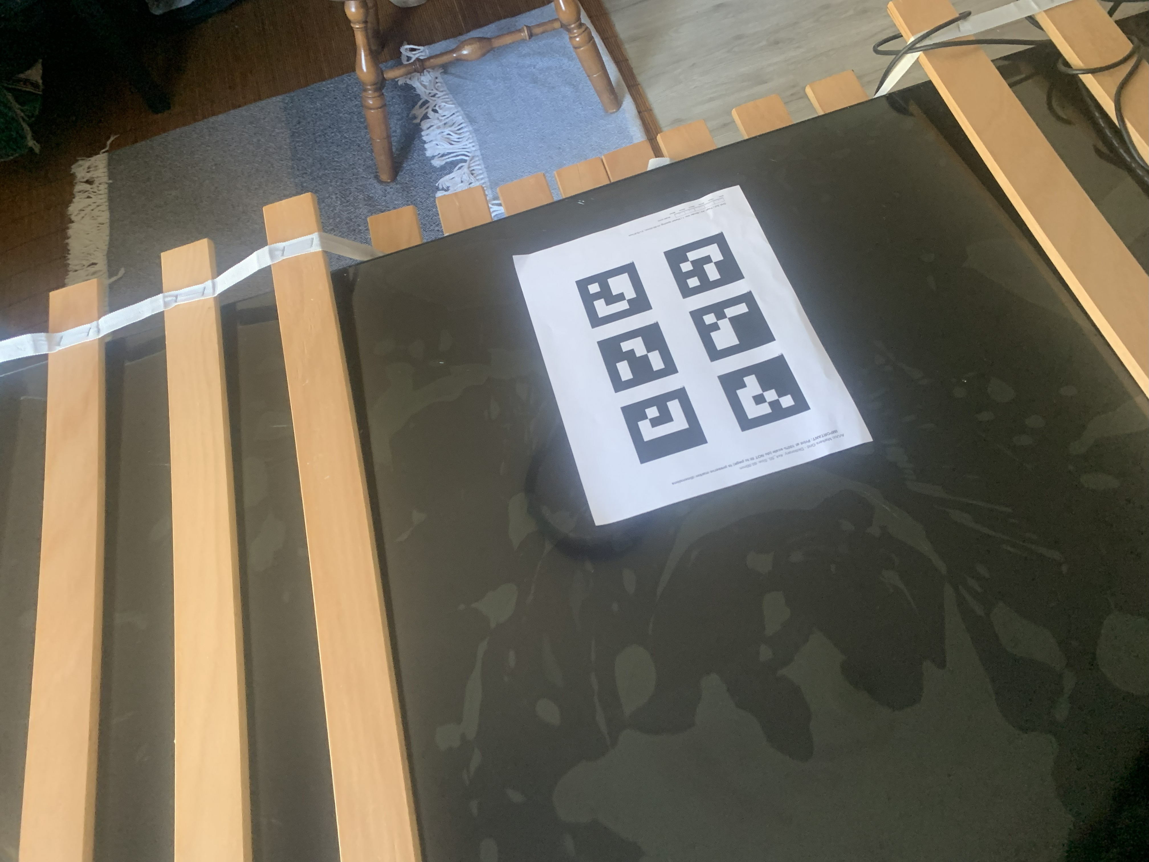
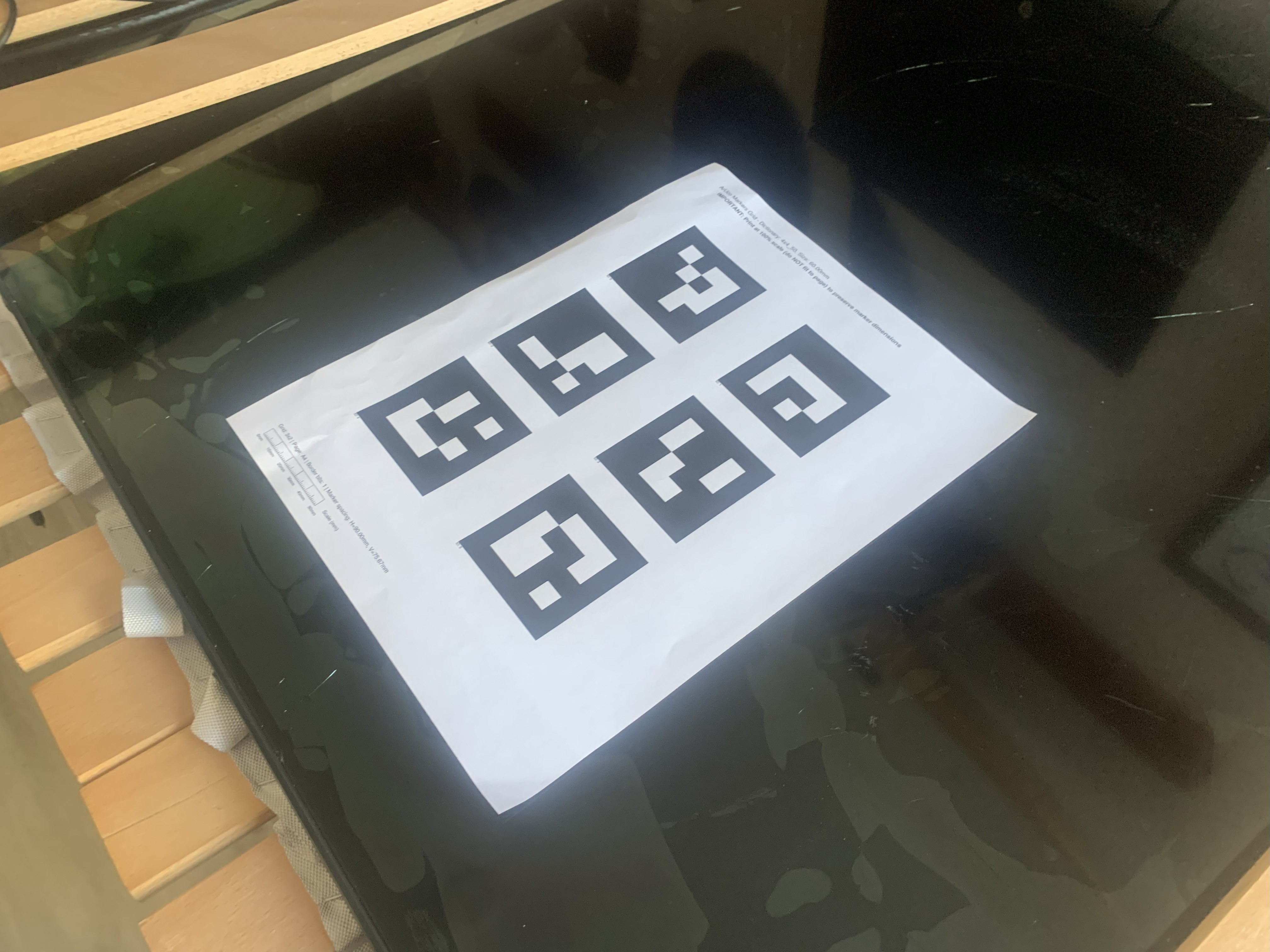
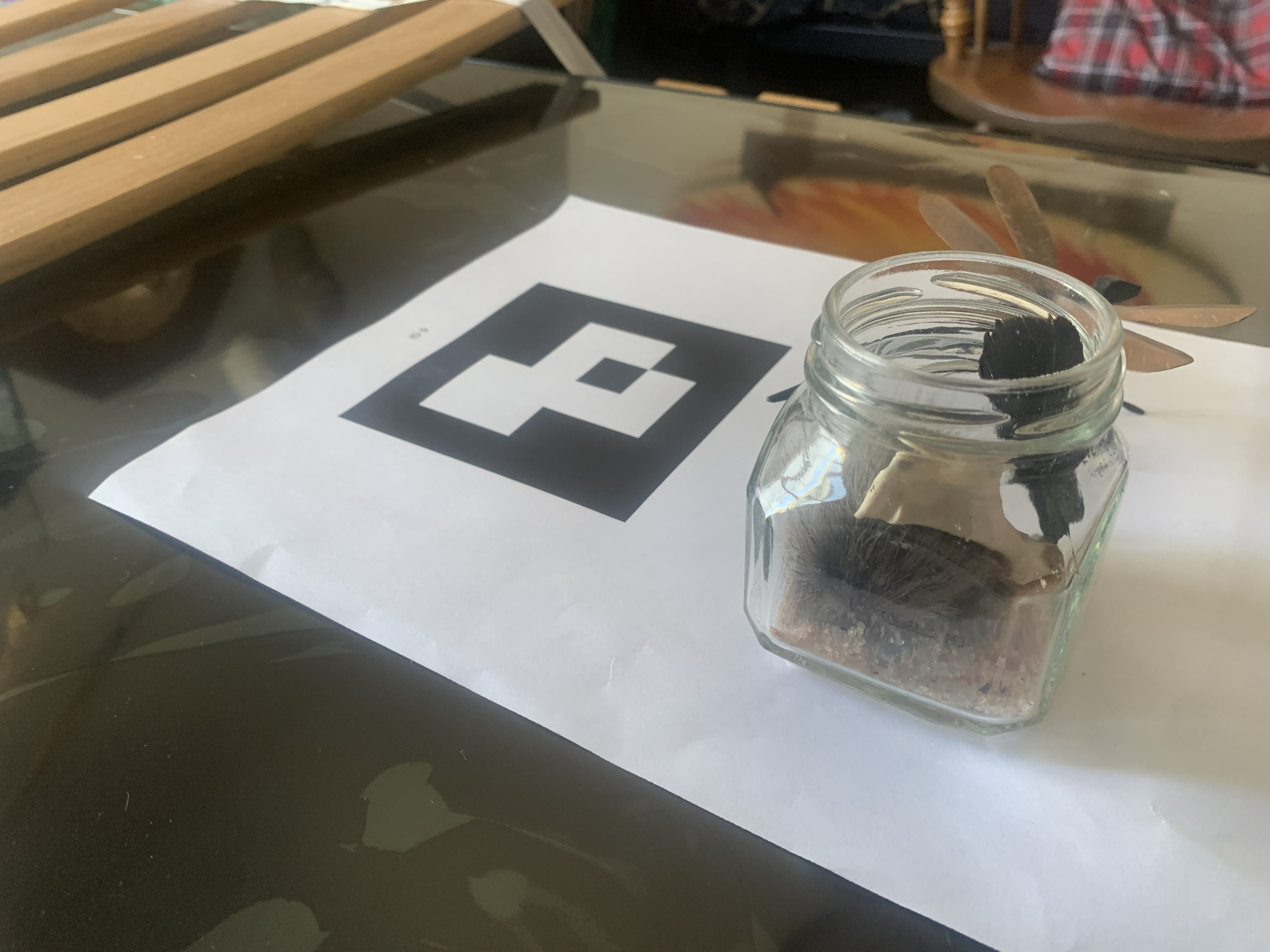
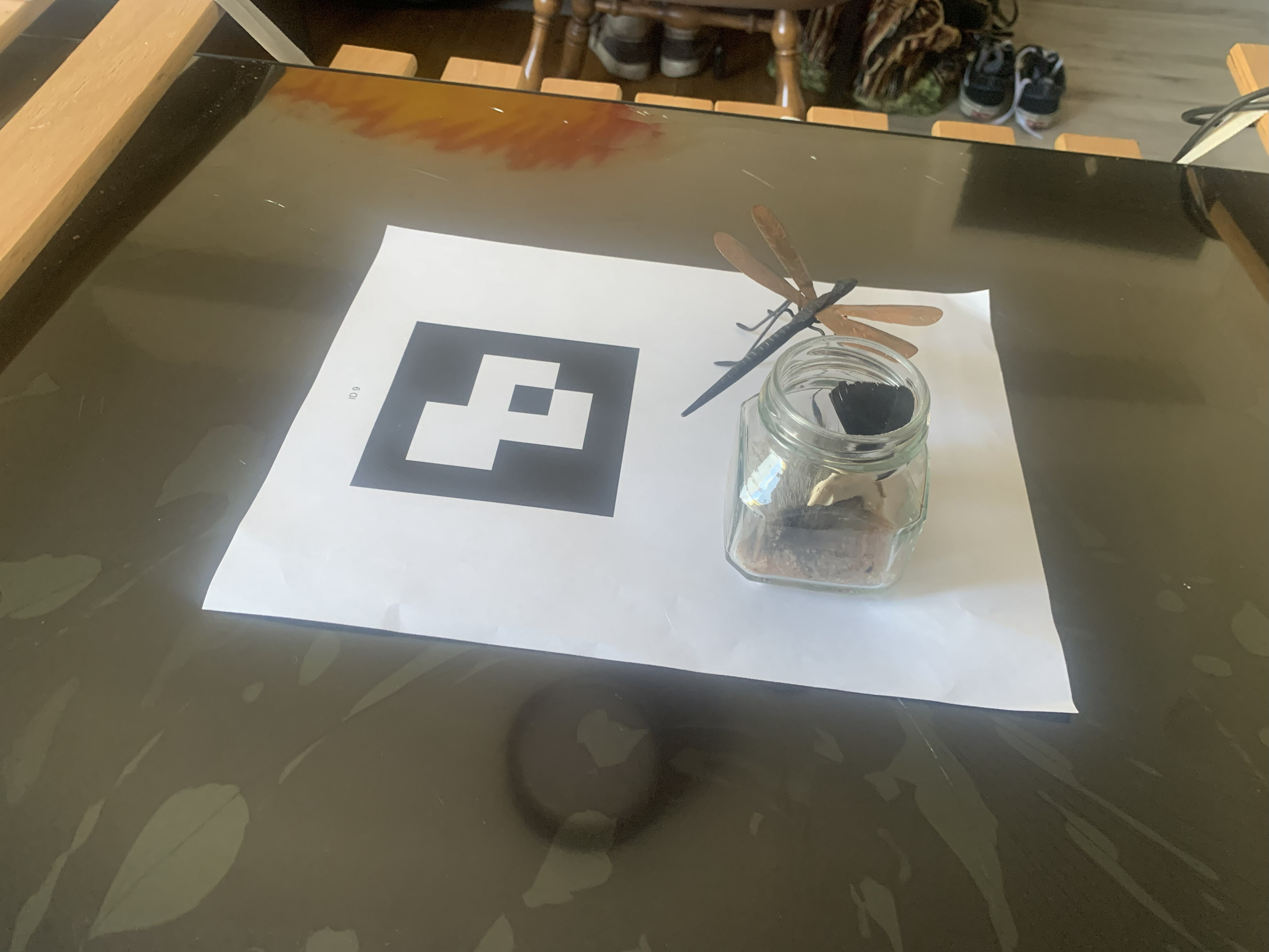
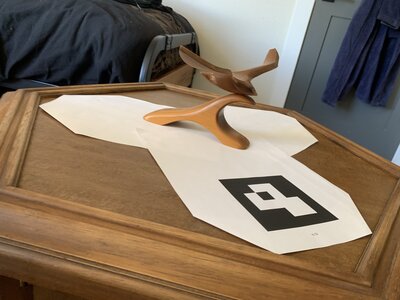
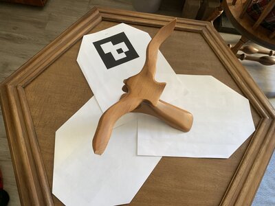
In order to create an effective NeRF we need a well-created dataset for the model to train on. Using a core piece of computer vision technology known as an ArUco tag we take a variety of photos in various orientations in order to get a sense of camera intrinsics - what types of distortion we see in the image of a camera based on the way the camera is built. We can then use these intrinsics to undistort the images we will use in our dataset before utilizing the ArUco tags once more in the creation of the second dataset - that which we are using to create the NeRF. This time the ArUco tags are used to solve for the camera position... which is absolutely critical if we are going to create a dataset of any efficacy.
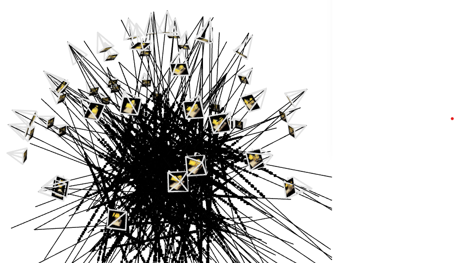
If we piece together all the images taken in this way into an external visualizer known as viser we get a composition similar to the following. What this represents is the position of each of the dataset generation images - the camera at the focal point of each of the four lines in the frame headed in the direction of the inversed scene. As you can see we attempt to get as many angles as possible surrounding a central scene.
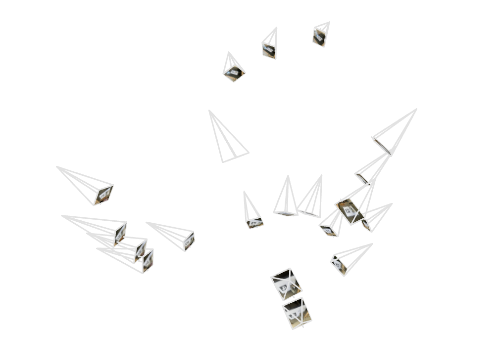
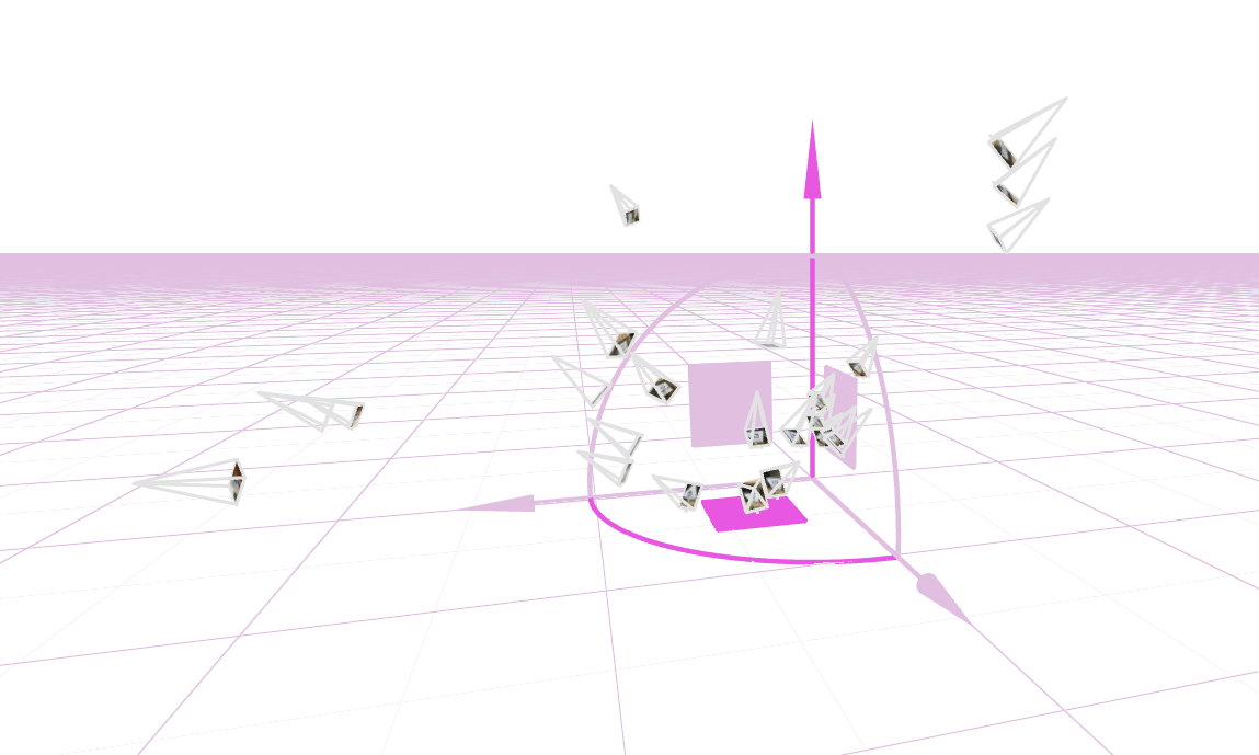
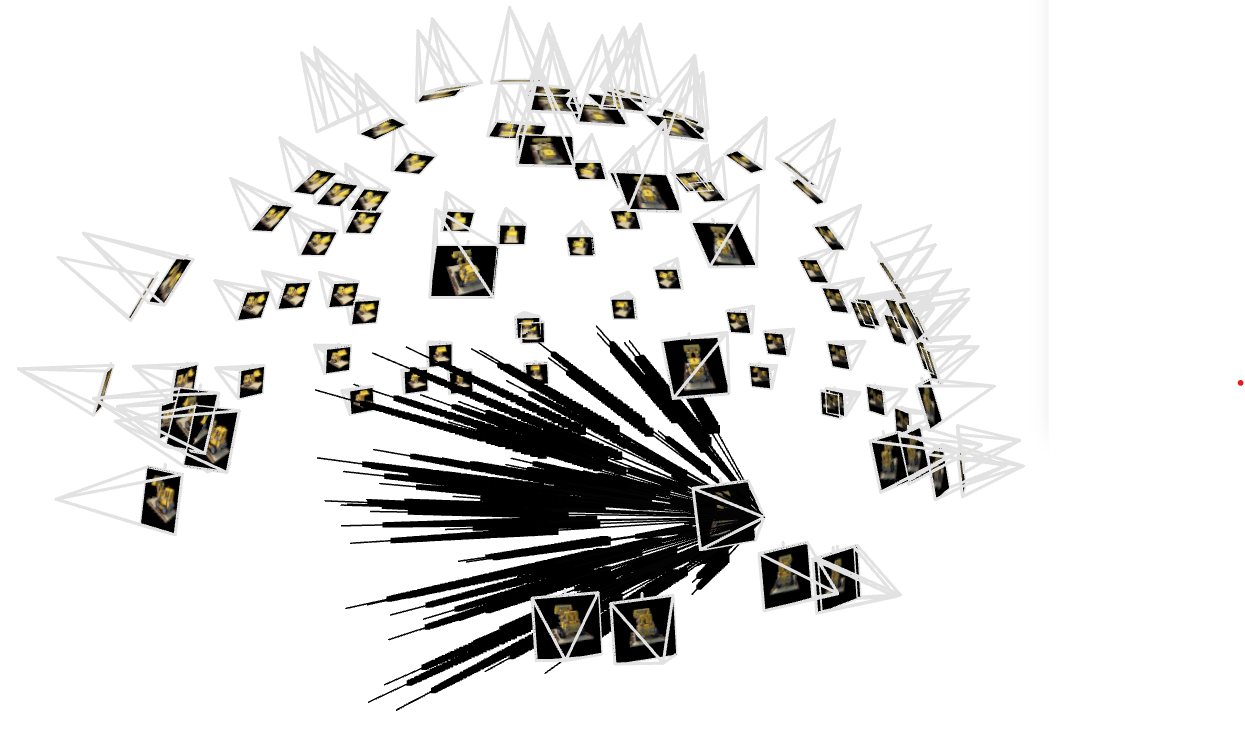
Except that dataset didn't quite work out, and I had to regenerate a second dataset to train my model on. Why? Because originally I had attempted to gather shots of varying depth in order to gain some sort of variety and ultimately those are not needed and instead cause the model to try and understand a further out scale of the scene than it should. Below is my second iteration of dataset and you can see that the frames are much more cohesive in depth and angle.
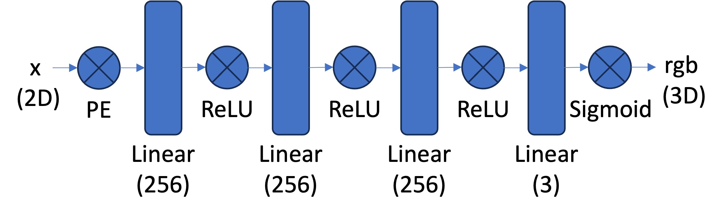
Whoo! Neural Networks. Those are some big buzzwords in today's world of modern ml. Let's begin by looking at the model architecture I implemented to get used to the nature of the assigned project. Below was the proposed model structure and I didn't really change much aside from varying the width of the three MLP layers to 128 nodes or 512. The model stayed with 4 trainable layers with ReLU activations and a final sigmoid activation to produce a color for the specific pixel we're trying to generate. Of interest is the PE - Positional Encoding - layer. This layer takes in the input x, y which lies in [0, 1]^2 scaled to the size of the image and through various L variables - in my implementation 4 and 10 - generates (4*L + 2) inputs instead of the original 2. This is done of various sine/cosine encodings within the original scale so the machine learning model can get an accurate understanding of where the specific pixel we're looking for lies. In order to update we used SGD - Stocastic Gradient Descent - with Adam update and a learning rate of 0.001.
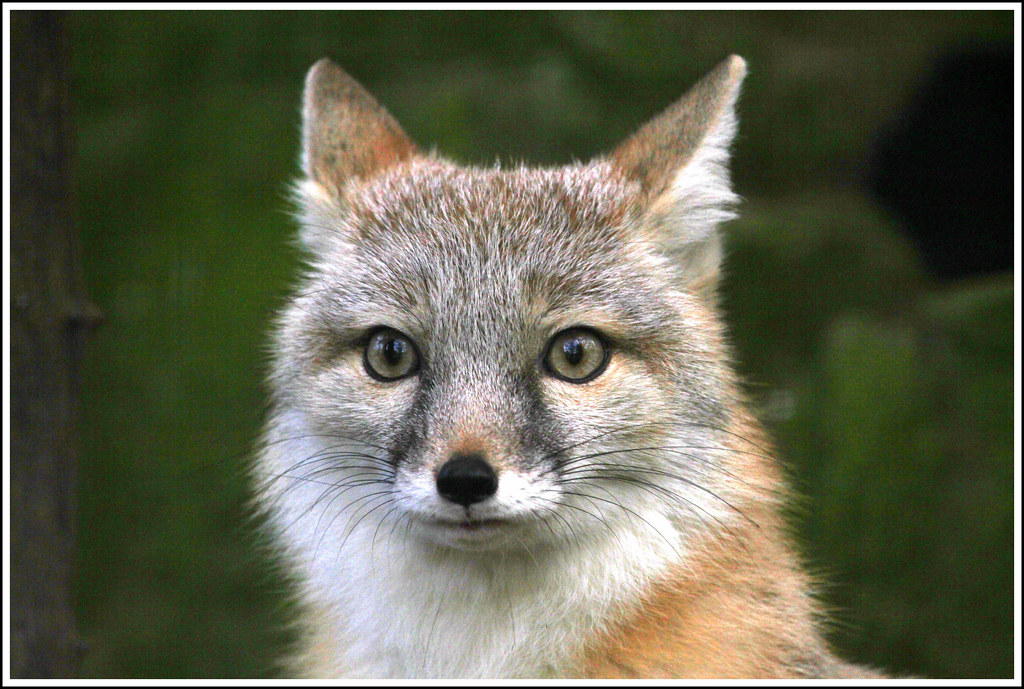
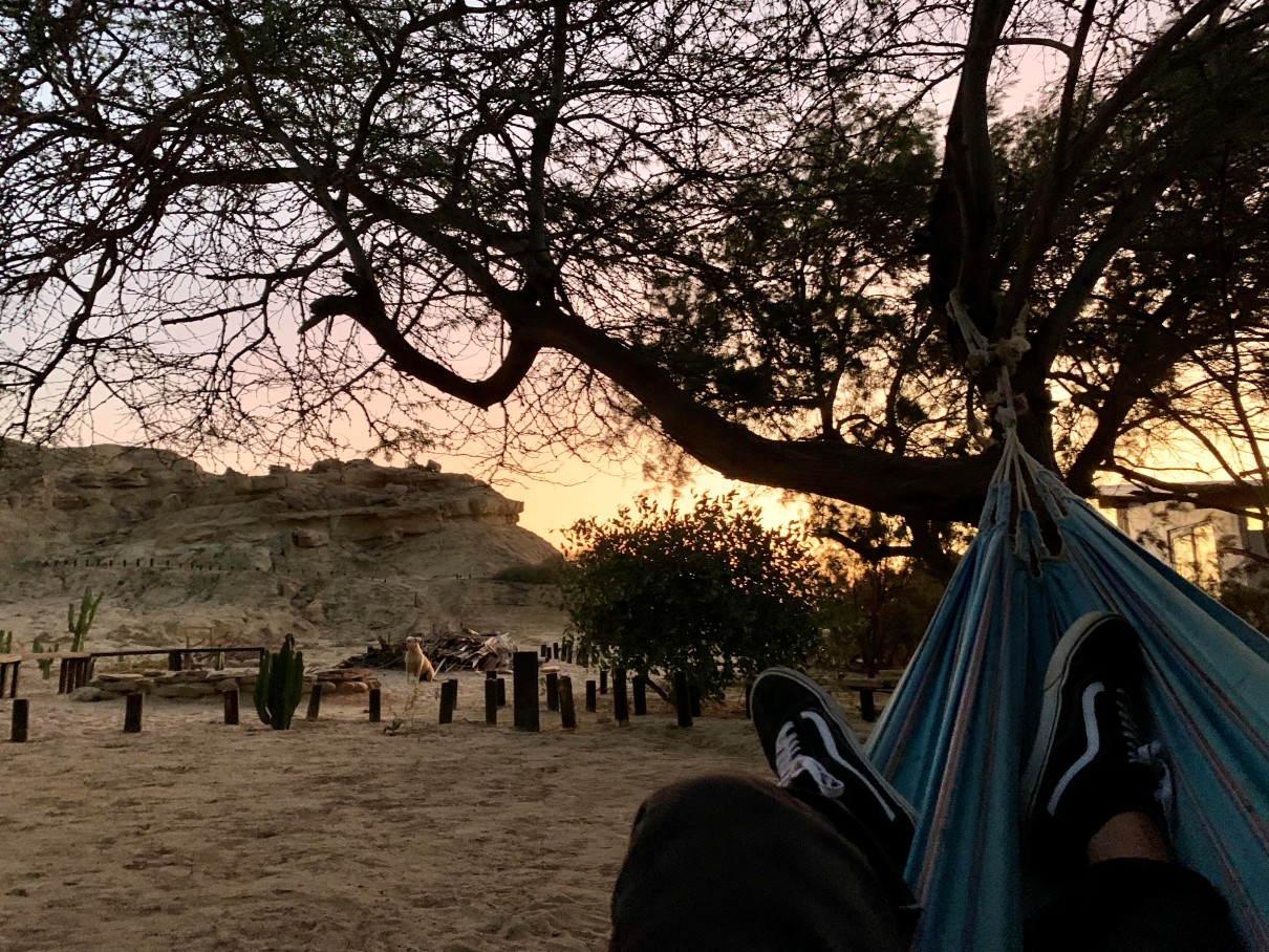
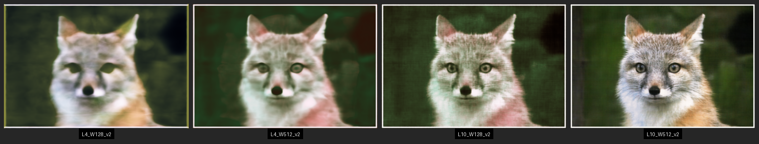
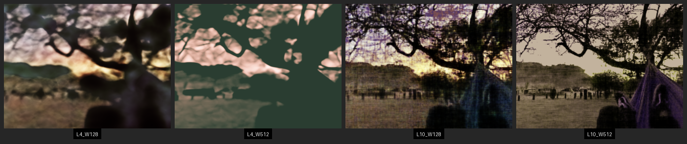
We also need input images to train on in order to replicate. Below are the two I used. The fox image was provided in project spec but the hammock image is one of my own. I tried to include an image with a lot of small details to confuse the model in test generation - the leaves of the tree. Both have a decent amount of low-frequency and high-frequency information. Let's see how the model performs!
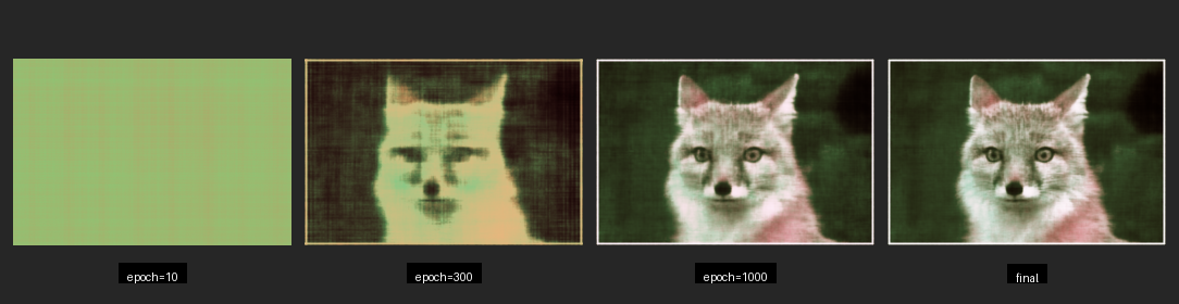
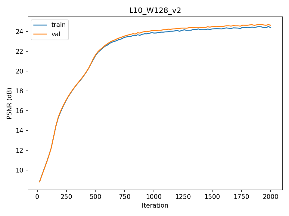
Below are eight different instances of model training on models of different hyperparameters and input images. To the right of the image is the PSNR - Peak Signal to Noise Ratio - curve of the image, where we can see how the model progresses in relation to epoch (or gradient step). We can tell that the models tend to slow down and stop improvement around epoch 2000 where we stopped training. We could have gotten more improvement but the goal is to familiarize ourselves with neural field training, not global optimization.
.png)
.png)
.png)
.png)
.png)
.png)
.png)
.png)
.png)
.png)
.png)
.png)
.png)
.png)
Let's look at the comparison between hyperparameters. It's immediately visible that a greater positional encoding - L - gives a much greater impact on image quality than an increase in layer width - W. Actually, I found increasing W to be often very frustrating. Not only did the model take much longer to train, it often got caught in a local optimum for colors and I frequently had to retrain it. The L4_W512 was especially susceptible to this as you can see even in the best training on the hammock image I had.
Let's go ahead and understand how the work done above translates to the 3D NeRF environment. Above we created a simple model and trained on the differences between an output pixel and it's correct color via mean least squares for loss. The most critical difference in the 3D environment is there is no such thing as a single pixel anymore. We are sampling across concatenated rays. This is rather hard to implement so let's understand the basics:
Rays from Pixels: We are operating in Camera2World convention and need to have a way to generate a ray from each pixel of images taken by our camera - after we have deducted the camera's intrinsics of course. To do this we first calculate the ray extending from the camera's point of origin and extends through the direction of the pixel seen - calculated as a vector with origin and normalized direction. This point origin and direction are then fed into the camera-to-world transformation matrix calculated as a rotation matrix (3x3) and transformation vector that get consolidated into a 4x4 homogenous coordinate transformation.
Sampling: Now, if we want to be successful in training a model, we must be able to sample points to compare our generated outputs against (again, we are optimizing our model via analysis-vis-synthesis). This means we have to sample points. But first we must create a way to sample rays from among the many images inside the dataset. We randomly sample images and from those images randomly sample rays. Parallelized because we're sampling many at once. Once we have rays we can go ahead and gather some sample points from along it by creating equidistant spacing (discretizing continuous rays) with a higher density nearer to the camera.
Dataloading: Theory is nice with sampling, but what about implementation? We need a dataloader that stays ahead of the optimization curve by providing batches (SGD) of presampled points to compare our model-calculated outputs against. Except we're dealing with actual pixels rather than rays. We don't have any 3D space. So what are we loading? Pixel Colors tracked with the ray that emerges from the camera in the direction of the pixels. And we calculate the ray with the next segment to be discussed. Visualization. And then the magic of backpropagation takes care of the rest with general model architecture.
Visualization: Both the most and least intuitive section - visualizing. For each ray we must load a volume most compatible. But we have many perspectives. The research done on volume rendering is perhaps the most critical area of NeRFs and where research went after it's original implementation - if curious read up on Gaussian Splats. To implement visualization we take all points sampled earlier and take a discrete sum of the color of that point with the transmittance of that point (density output in model) multiplied by the ratio of the transmitted light that actually reaches that point, as in not blocked along the way.
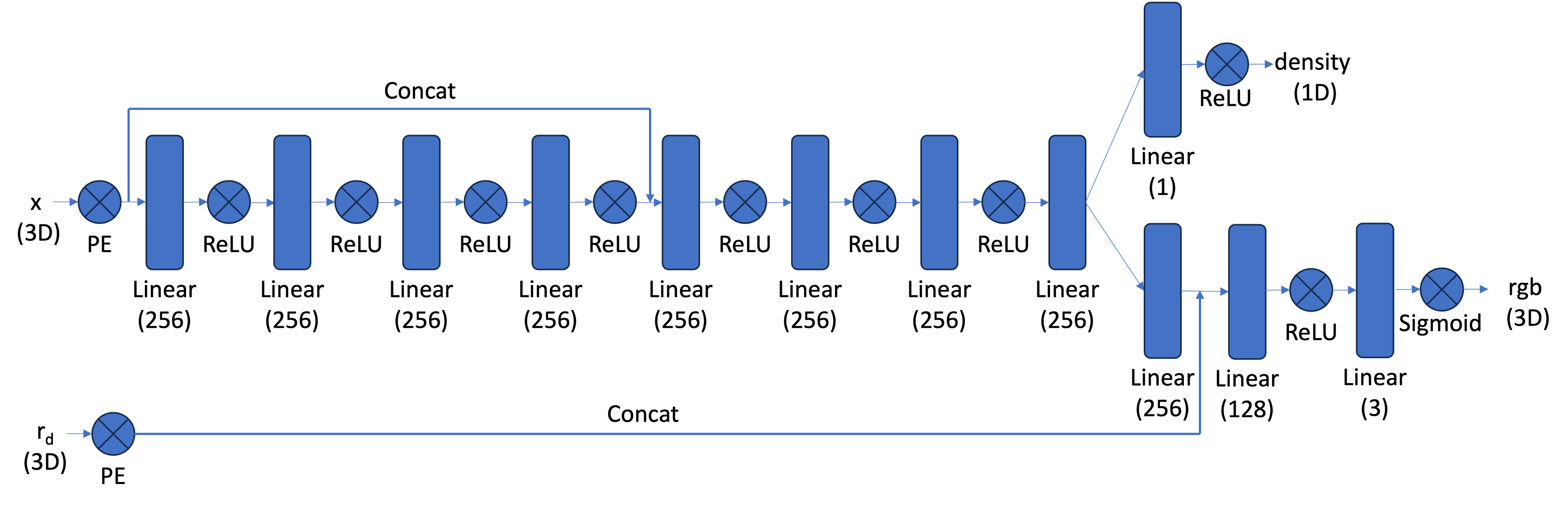
Model Architecture: Our model architecture (pictured below) is a lot more complicated in the 3D NeRF process than it was with 2D Neural Fields. We have more inputs, the points in 3D space and our 3D viewing angle; we have more layers, 8 in trunk splitting into two separate paths; we have more concatenations and outputs and a hellova lot more weights to train too. This architecture was provided in project specifications but implementing required a detailed understanding of how to create the forward pass (especially where concatenation and splitting was involved) to recieve outputs on both separate trains. We trained the model via backpropagating through this model architecture and optimizing with Adam and Stocastic Gradiant Descent. The learning rate for my model is 0.0005.
In this setting we also need images to train on, but rather than a single static image we need a scene and many captures of that scene, each capture being a 2D array of pixels otherwise known as an image. As is traditional for neural nets this needs to be divided into training, validation, and test sets. We must also have a way to iterate through these and test that we are training correctly. I spoke a bit about it above but this is the main function of the dataloader. Below are some visualizations of this dataloader in action using viser as we did in camera calibration. As we are using a standard dataset - lego_200x200.npz - we have camera intrinsics already solved out for and calculated. So this section is a way for us to see how the dataloader loads each scene. Or rather samples and loads a set of individual rays for the model to train on.
We have now found ourselves in the process of training this model upon the lego_200x200.npz dataset. In order to do this all the code had to be transferred from vscode with git to google colab to take advantage of good gpus. However, to not waste hours andhours on trainign time this proved to be worth it. Below we can see a set of training images from the model as it developed and the PSNR curve of that model on the validation set.
Our final task on the given dataset is to generate a novel visualization of our lego truck in a circular motion using the trained Neural Radiance Field. This is the primary function of this technology, the creation of novel views from existing datasets and scenes. The below image shouldn't be incredible in terms of quality but is more a proof of concept. There are ways to improve this quality that have developed in recent years but they were not implemented here. Something to notice with both novel scene recreations are the black lines through an otherwise well-formed and formatted model. This is likely the result of the model not understanding the inputs at certain angles and defaulting the density of points seen at those angles to background. If we take a look at the training data we can see the images are taken at regular points around the sphere with regular internal angles. This means there are may be gaps in that system. Another possible explanation would be areas of frequencies congruence on positional encoding where the model doesn't know how to generate a proper color. Or perhaps they represent the highest frequency the encoder can create as you can see they are generated with somewhat of a sine wave pattern. Regardless, the model can clearly capture much of the internal structure of the lego truck.
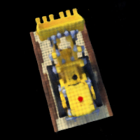
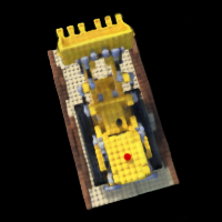
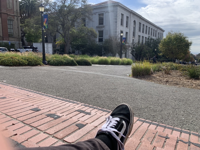
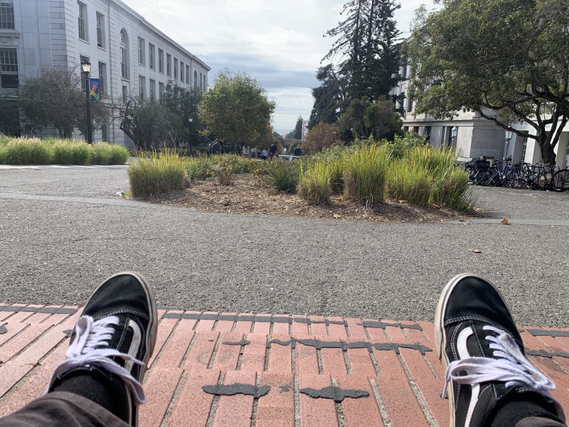
In this second part we are going to train a model on a dataset of my own creation - bird_dataset_v2.npz. This dataset had to be retaken after the initial attempt produced abject failure. It's not perfect here, but we have some sort of image render that can be seen to correspond with the original scene - as you can tell via the coloring scheme. Below we have a couple examples and their comparison with the first set of images I took. Above in Camera Calibration you can see the difference in frustrum but we'll also look at the images themselves below. A little added description - Object_3D were taken and not reduced, so were originally of size (4024, 3018) from the iPhone camera while bird_dataset_v2.npz (notice the much smaller size of the font) was all of images that were (400, 300). They also had much greater contrast and were instrumental in cleaning up one part of my room.
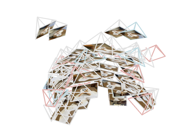
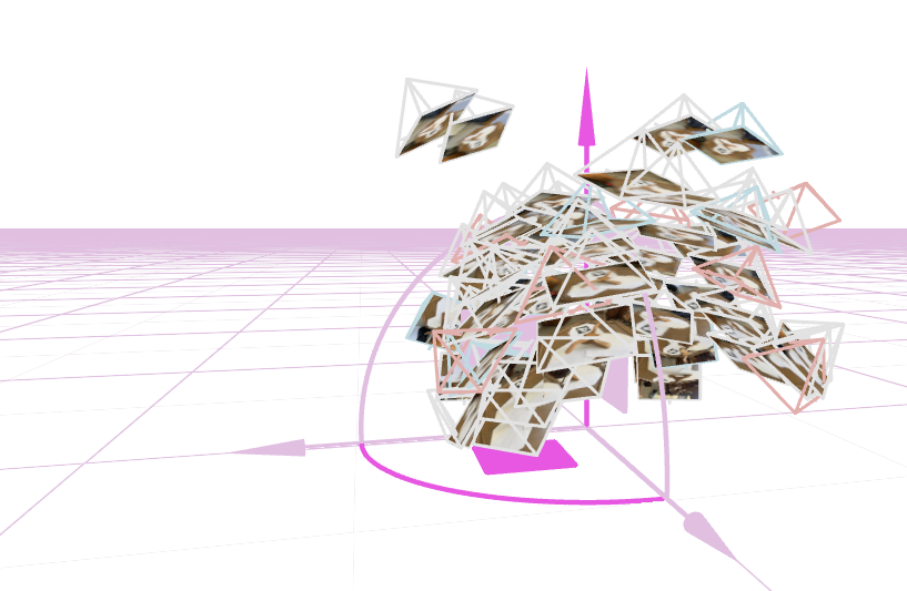
Beautiful. Now let's look at the frustrum projections (similar to the lego_200x200.npz dataset). As we can see the rays all correspond with one central area that was scanned from many different angles. I went ahead with this dataset and removed any outliers that had a recalibration_px amount for their ArUco-scanned camera-to-world conversion matrix for the original image from the location derived from pnp (structure from motion). This means that the final dataset ended up excluding any scenes that had a high amount of noise (>3 r_px) in their inherent data - be it from motion blur, miscalibrated ArUco tag because of paper with lifted edges, or very obtuse angles in the specific shots. We then have a cameras that capture a scene simialar to below.
Let's train this model! Training went a lot longer this time around as I figured out how to let the model just sit on colab's A100 GPU rather than my laptop's CPU (first runs on learn_2d), laptop's GPU (Nvidia GTX 1650 Ti), or initial runs on colab that cut short due to my laptop shutting down for sleep, aborted psnr curves, or a babied final run for lego_200x200 that I sort of wateched tick down for an hour for 10000 epochs. Here I set the run with updated colab cells, let save into drive at checkpoints to be potentially reloaded, and let cook for 3 hours while I went on a walk to the park. I checked once halfway and saw some issues but kept the run ongoing. This model ran for a total of 20000 run epochs - twice as long as the lego_200x200 dataset. However, the model architecture was kept the same. Most of the changes in code were made to the Google Colab cells for long training times, checkpoints, and data cohesion. Below you can see intermittant captures of the model training upon bird_dataset_v2.npz:
.png)

.png)
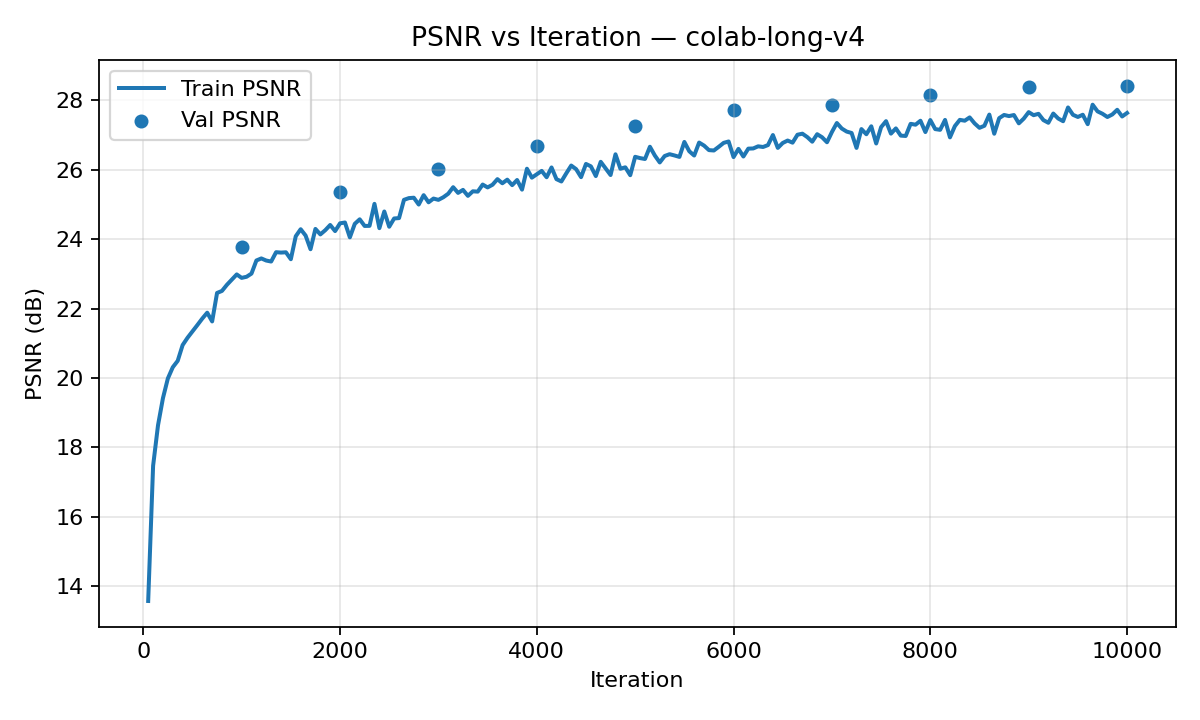
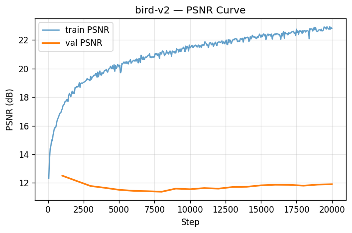
All well and good, but does the model capture the underlying structure of the data? As we can see in the PSNR curve, not quite. While the training PSNR achieves a pretty high standard (blue, around 23), our validation PSNR lags far behind (orange, barely crossing 12). There are a couple of potential reasons for such; the first is the presence of a non-dark background in my training set. This background means any validation data must recreate a background that is entirely not suited for the frame. This also means, since background has the potential to be unique to some frames for specific angles, that some frames are optimized to include slices of their further-off background throughout the scene as there are few corresponding cameras to give depth to that far-off point. There are multiple other alternate explanations for the model's overfitting to training data of course - the extent of the run, model hyperparameters especially including positional encoding depth, vanishing gradient during training to name a few. But suffice to say this model didn't capture the true signal and got lost in the noise.
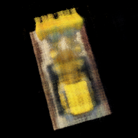
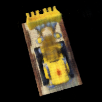
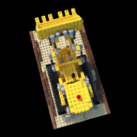
Finally finally, let's look how the model created off bird_dataset_v2.npz performs when viewed from multiple angles in the creation of novel scenes - the entire point of Neural Radiance Fields. While my model was not quite successful at recreating the structure of the bird or any fine details, we can capture a vague understanding of the placement of colors within the scene. Additionally, if you pay attention to the render on the left you will occasionally see a brown bird fly across the scene to the right. It's pretty faint, but it's there and it comes around once a cycle. So somehow we still capture a bird. Upon closer inspection of the scene by zooming in and taking a more vertical angle (the render to the right), we can see how the point-clouds actually look. At some frames we are even within what the model considers the ground plane. I think the white nebula I found was pretty cool and deserved a final spot within this project.

Mosaic Stitching
In this project we went through the process to feature match seperate images, compute homographies betwen these sets of points, create a large canvas capable of holding more than one image, warping one image onto the plane of the other, and blending the two images together using laplacian stacks. This whole process generates what can be seen as an "image mosaic", a composition of multiple photos that captures more of a scene than one photograph would be able to and in the process reveals more of what our human eyes are able to capture. These compositions are also artistic and can reveal multiple perspectives in the same scene.
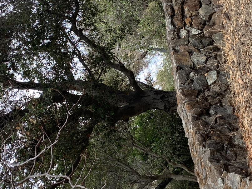
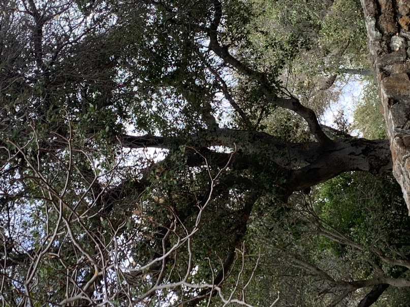
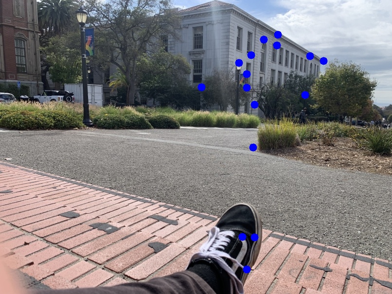
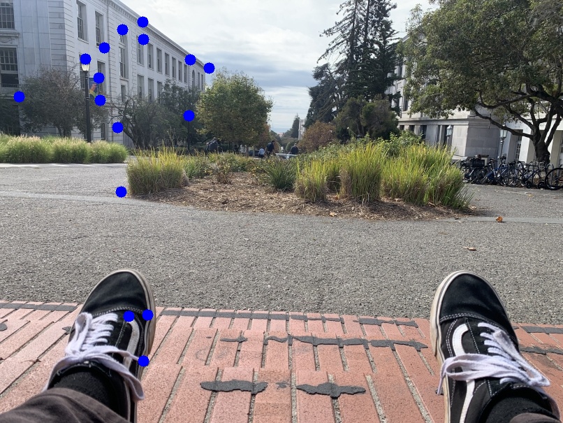
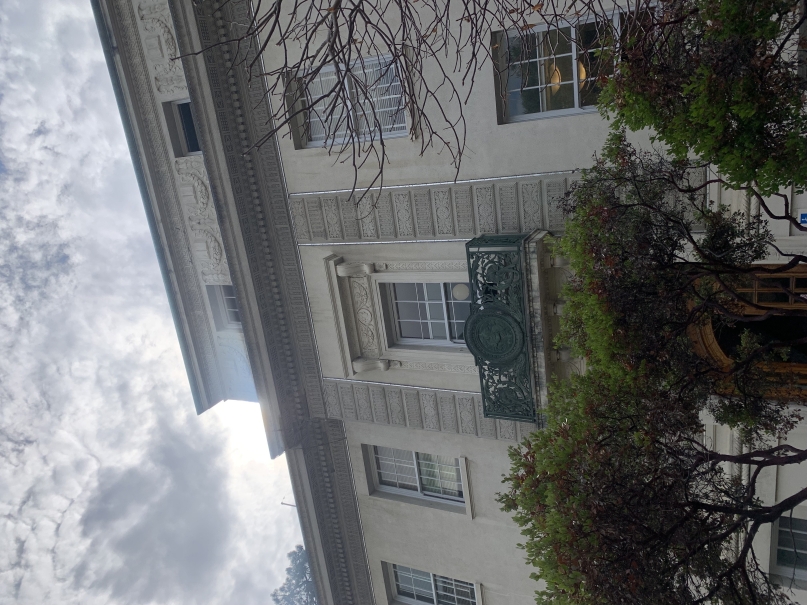
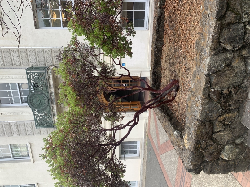
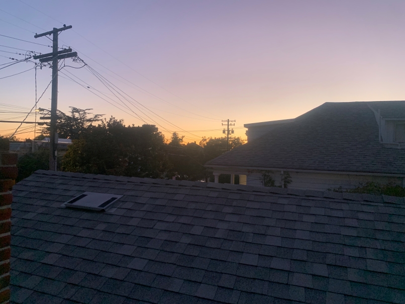
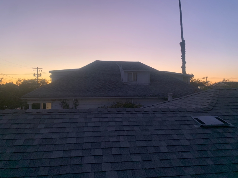
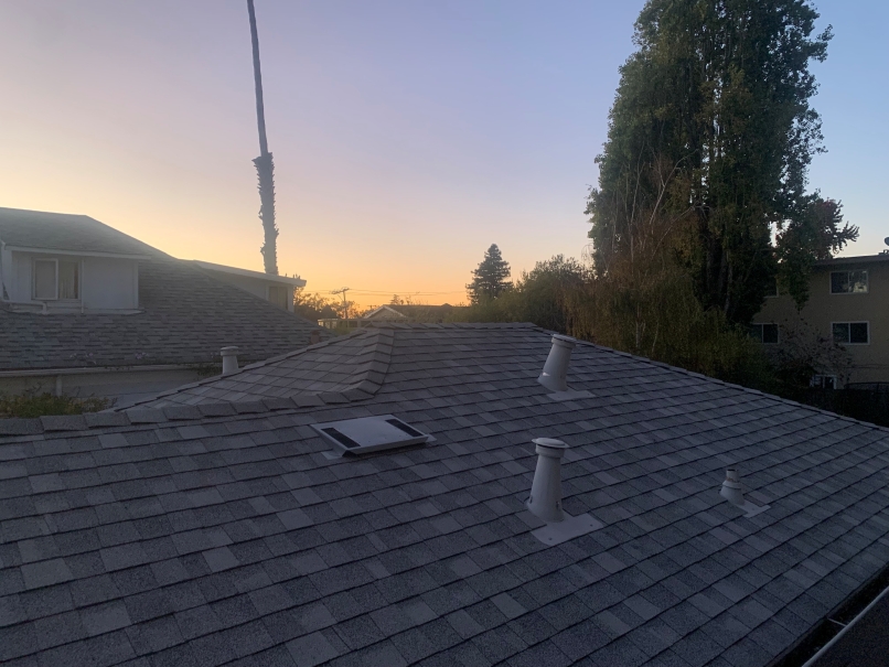
Below are a series of images taken with the intention of composition. In order to do so these photos are taken while only rotating around the camera. This means that the pencil of rays the camera can capture and project remain the same as the boundaries of the image change between photos of left, middle, and right.
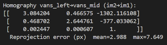
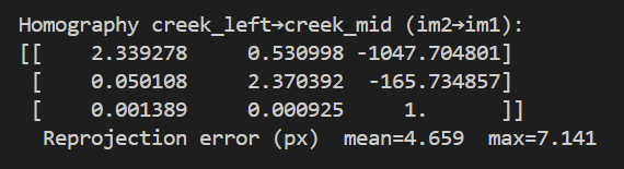
In order to compute the homographies of the images I intend to project, I first need to do ungodly amounts of point and click in order to find correspondance points between the two images. Then, for each such point (x,y)→(u,v) I build two rows in my least squares solving matrix A:
xh1+yh2+h3−uxh7−uyh8=u
xh4+yh5+h6−vxh7−vyh8=v
Stacking all points gives Ah=b, with h=(h1,…,h8)⊤ and h9=1 solved via least squares.

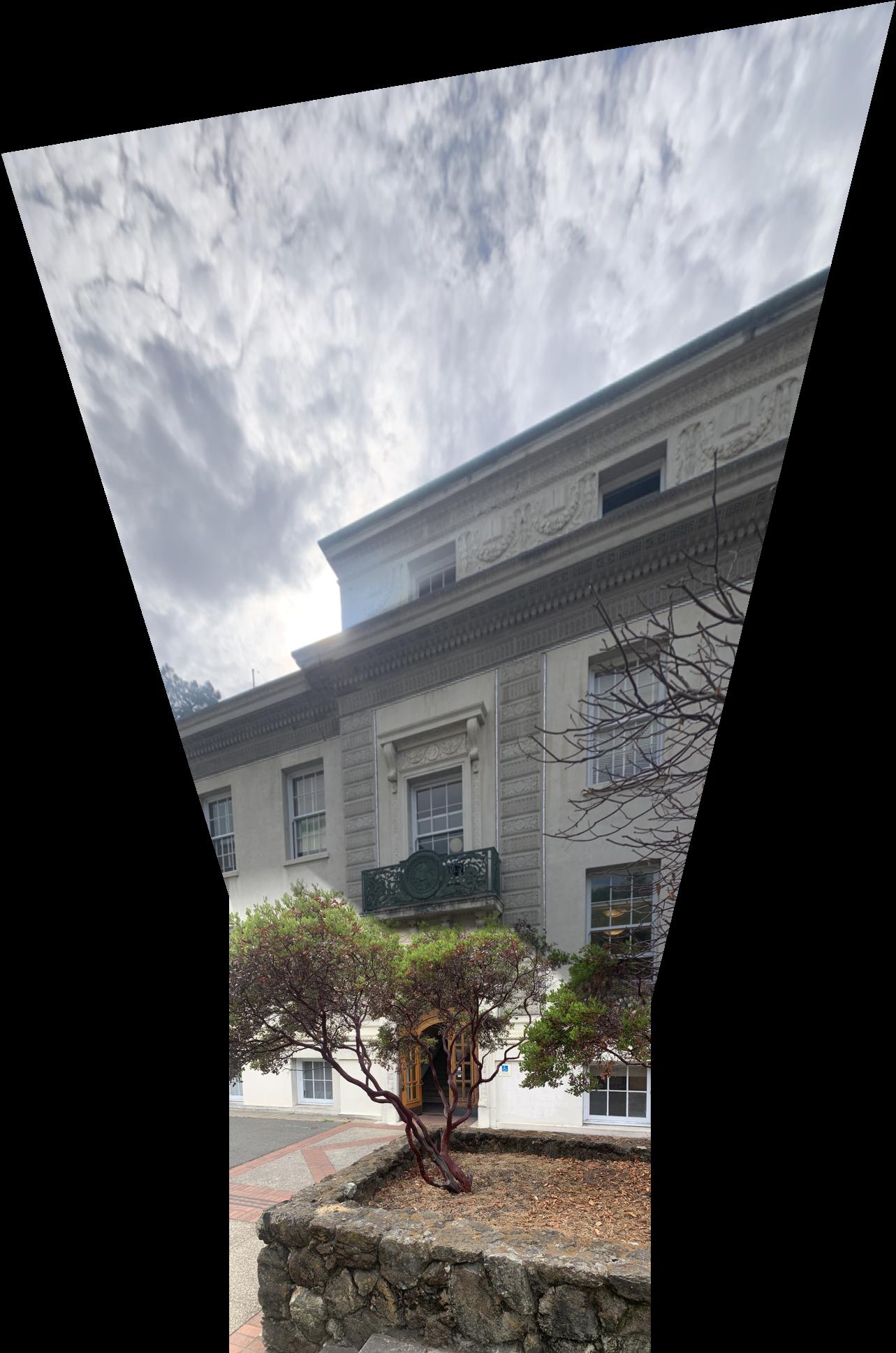
We are now in the stage of image warping, but before we do that we need to create a valid canvas and warped plane. Once that is there we inverse sample from the original image pixel by pixel... or vectored over all pixels at once if you can't stand the long wait times for this operation to run. And with the point coordinate of the original image we either round to the nearest whole pixel (nearest neighbor) or bilinearly weight the four closest pixels depending on how close each is (bilinear). Nearest Neighbor operates faster, but bilinear sampling has a higher resolution and looks closer to the original image. Now upon vectorizing this entire operation, nearest neighbors has the benefit of being far simpler to code as well... but that will not deter me! At this point we are also able to Rectify any image, being able to rectangularize any portrait or other rectangular object within the image to be rectangular on the final screen. That process is shown below as a demonstration of nearest neighbor vs bilinear warping. You can immediately tell bilinear sampling is far superior in terms of visuals.


The last stage of computing an image mosaic is going through the process of creating stacks of both images to be warped and blending them together one layer of stack at a time. Because the two examples are of three image mosaics I went and did both "halves" seperately first finding the left/middle then adding the right.
Below we have a final array which has the images stacked vertically. Here it's far more obvious to see the seam between images. This is because the top photo directly includes the sun and therefore has its brightness scaled to such while the bottom image does not. There are possible rectifications for such but I decided not to include them in the build.
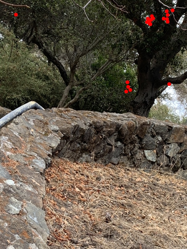
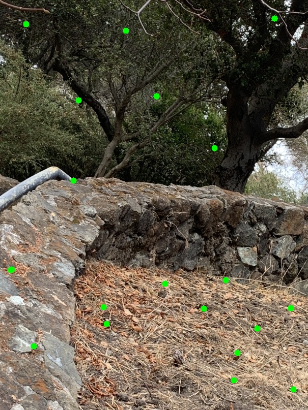
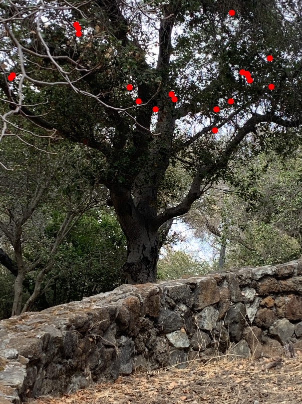
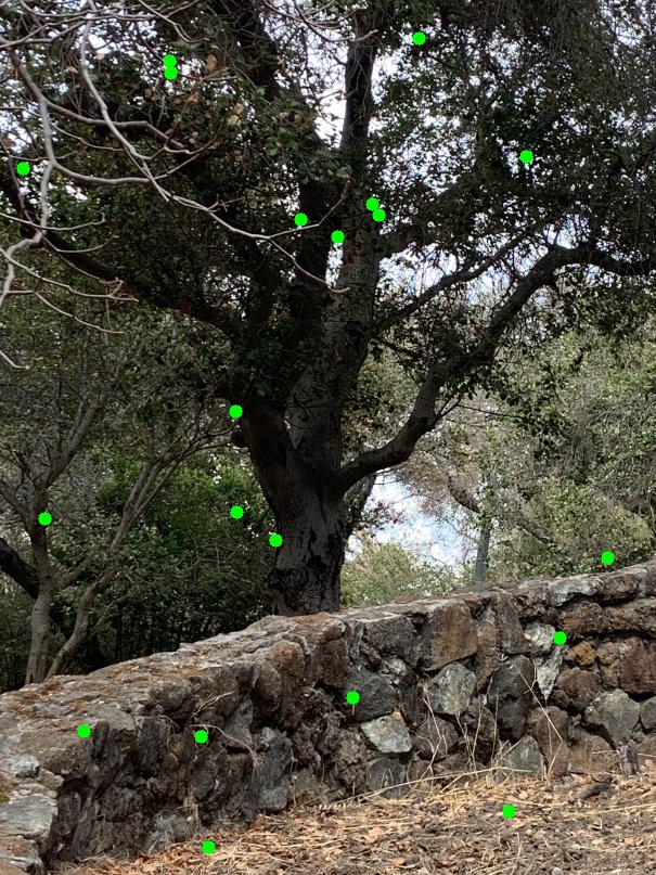
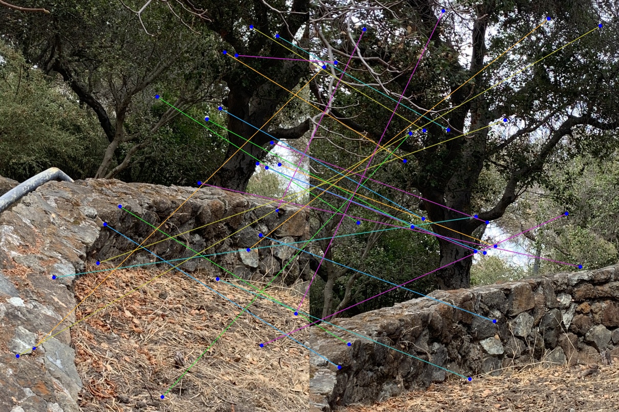
The first part of feature matching is the process of detecting segments of the image which have the possibility to be found image to image. This is done through the Harris Corner Detection method. However, the Harris method can be seen to leave these corners/features bunched up together in similar parts of the image where there is a lot of identifiable characteristics (seen below in red). We implement ANMS in order to expand the radii between these points. This is done by creating a weighted list by radii and taking the first N corners from that sorted list (seen below in green). As you can see this process is vastly superior in spreading key points throughout the image.
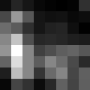
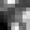
For each key point gathered in the Harris Corner method we need a way to match with a corresponding corner of the image to be matched with. That means we need descriptors. These are gaussian blurred samples reduced from the surrounding 40x40 pixels to become 8x8s. There are ways for these to be size and rotationally invariant but they are not implemented here. Below are some examples of feature descriptors.

Now begins the process of matching these feature descriptors between images. This can be done rather simply with an L2 Norm. Far more of the work goes into eliminating outliers in this process. We first eliminate all matches where the distance between the image and the closest is not too much less than that and the second closest. This helps some, but moreso allows us to iterate less with the RANSAC protocol. RANSAC being a miracle worker computing the optimal set of inliers for the dataset of potential matches. RANSAC does this by iterating thousands of times through a combinatorial set of possible matches choose f4, computing a potential homography on such, checking how many potential match pairs can be explained by this homography, and updating inliers if this number of potential match pairs is higher than found before. It works because probability.


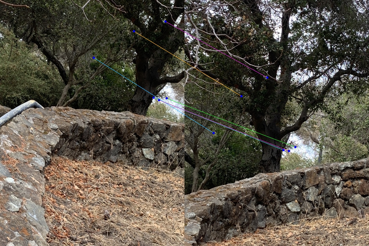
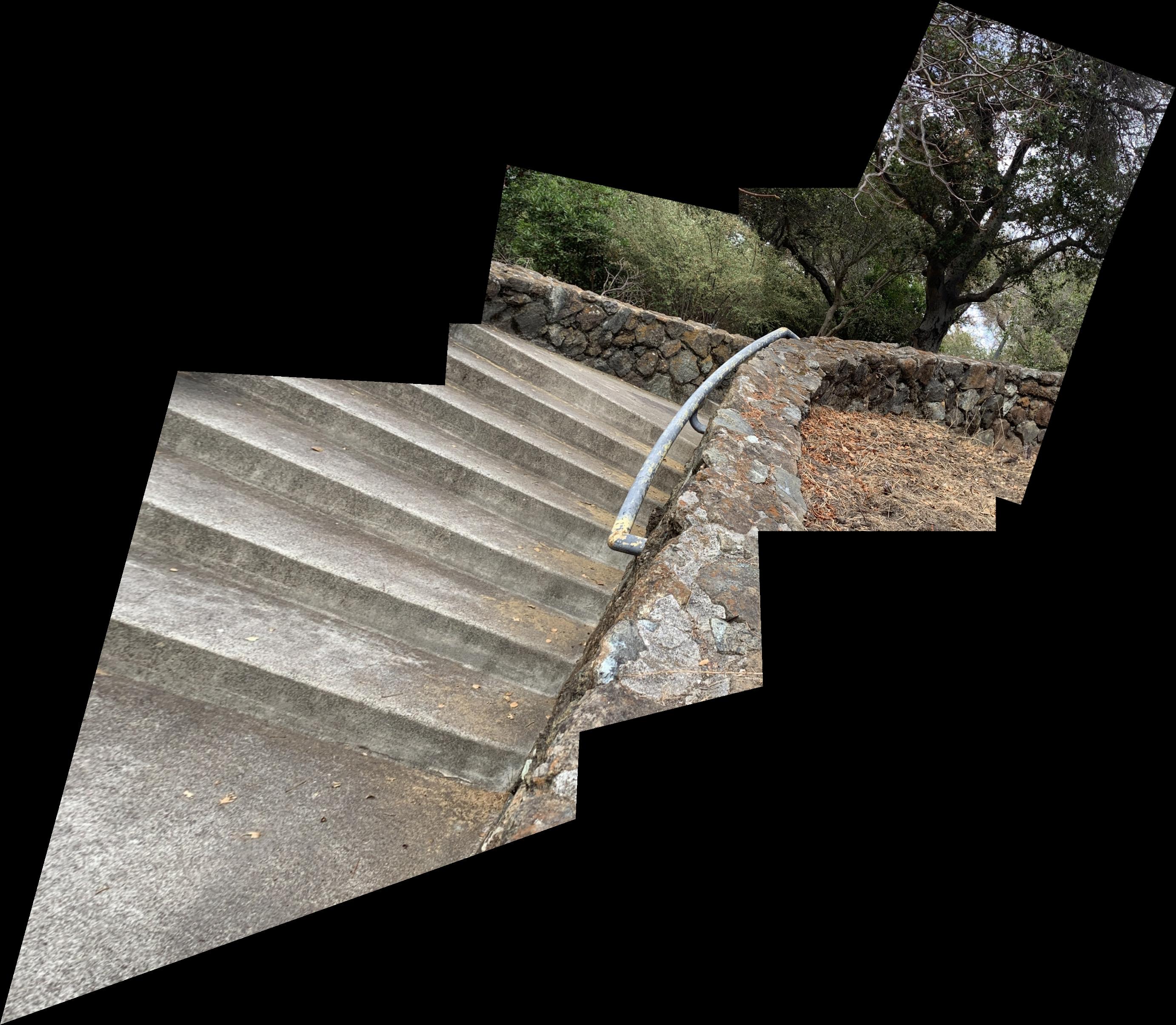
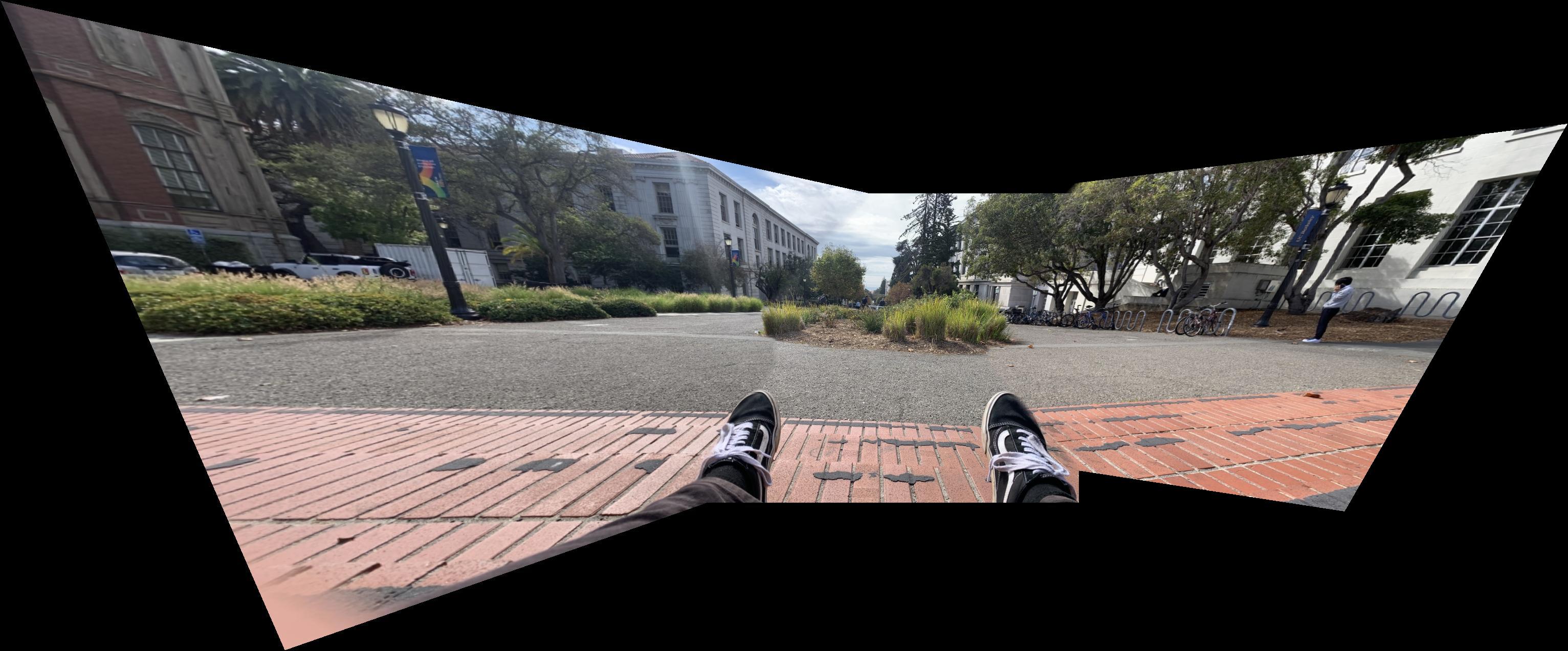
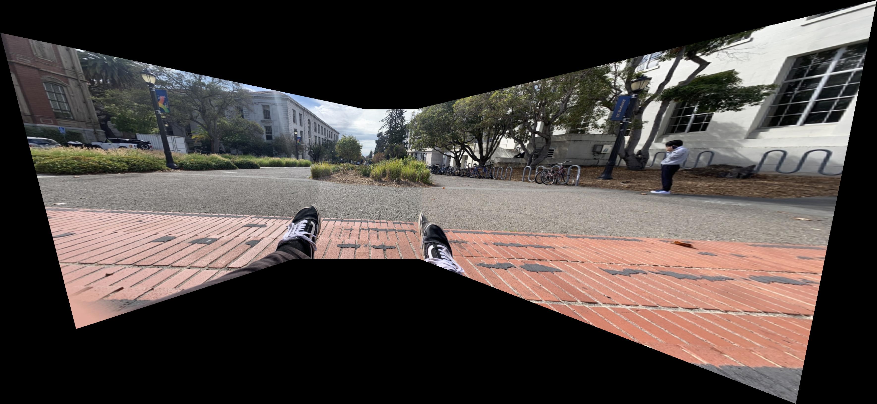
We've come to the final segment of this project! Running the automatic feature matcher along with mosaic composition as defined in the first half of this project. Below I've compared Vans Mosaic Manual with Automatic along with generating a Rooftop Mosaic Automatic. Some commentary on the differences between Manual and Automatic: At first it may seem like the feet are being improperly computed in the Automatic but as I was trying to fix that I realized the Manual actually had a much more egregious error - the brick step suddenly veers off at an angle! In computing a manual correlation I focused far too much on the identifying components of my shoes and had the image overcorrect for some small changes I made in foot placement between images. In contrast the Automatic took far more care in having the background correct. Something to note for mosaic composition is that body placement is hard to get the same between images and alterations are far more prominent the closer the correlated features are to the camera.
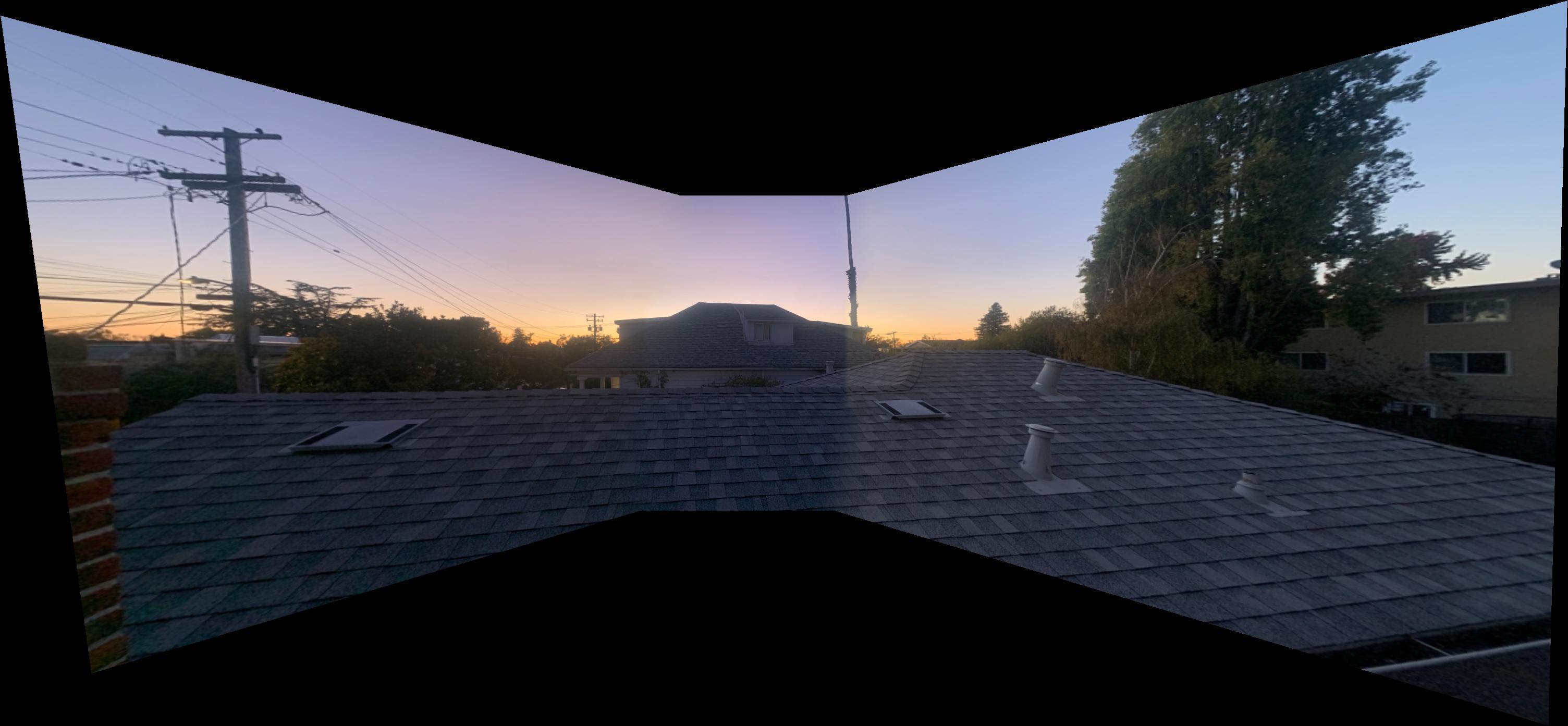
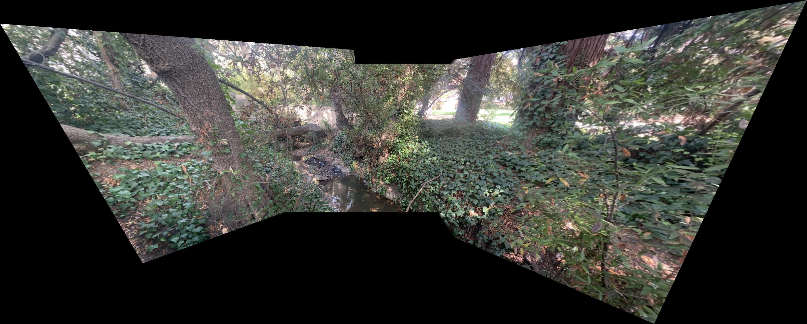
Below is the final personal ask for this project. Could I create a function that passes in many different photos in a different orientation than before and have a function call take care of everything all at once - iterating outwards from a center projection base splining each further mosaic section into an expanding canvas. As I write this it's incomplete. The image will speak if I have done a good job. Cheers for reading.